Seurat workflow
Bernd Jagla
bernd6/7/2020
Source:vignettes/pkdown/SeuratWorkflow.Rmd
SeuratWorkflow.RmdIntroduction
Please see the Seurat workflow for a more in-depth workflow.
https://satijalab.org/seurat/v3.1/pbmc3k_tutorial.html
This workflow uses a dataset of Peripheral Blood Mononuclear Cells (PBMC) freely available from 10X Genomics. There are 2,700 single cells that were sequenced on the Illumina NextSeq 500.
download data from https://s3-us-west-2.amazonaws.com/10x.files/samples/cell/pbmc3k/pbmc3k_filtered_gene_bc_matrices.tar.gz
library(plyr); library(dplyr)
library(Seurat)
library(patchwork)
library(SCHNAPPs)
library(SingleCellExperiment)
# Load the pbm dataset
pbm.data <- Read10X(data.dir = "~/Downloads/filtered_gene_bc_matrices/hg19/")
# Initialize the Seurat object with the raw (non-normalized data).
pbm <- CreateSeuratObject(counts = pbm.data, project = "pbm3k", min.cells = 3, min.features = 200)

pbm[["percent.mt"]] <- PercentageFeatureSet(pbm, pattern = "^MT-")

## in case of human samples:
# pbm <- CellCycleScoring(
# pbm,
#   g2m.features = cc.genes$g2m.genes,
#   s.features = cc.genes$s.genes
# )


scEx = as.SingleCellExperiment(pbm)

colnames(colData(scEx)) = c("sampleNames",   "nCount_RNA",   "nFeature_RNA", "percent.mt" , "ident"       )
colData(scEx)$barcode = rownames(colData(scEx))

rowData(scEx)$Description = ""
rowData(scEx)$id = rownames(rowData(scEx))
rowData(scEx)$symbol = rownames(rowData(scEx))

pbm
## An object of class Seurat
## 13714 features across 2700 samples within 1 assay
## Active assay: RNA (13714 features, 0 variable features)
pbm <- subset(pbm, subset = nFeature_RNA > 200 & nFeature_RNA < 2500 & percent.mt < 5)
pbm <- pbm[-which(rowSums(pbm)==0),]
pbm <- NormalizeData(pbm)
pbm <-FindVariableFeatures(pbm, selection.method = "vst", nfeatures = 2000)
top10 <- head(VariableFeatures(pbm), 10)
all.VariableFeatures = VariableFeatures(pbm)
all.genes <- rownames(pbm)
# Why do they scale on all features???
set.seed(1)
pbm <- ScaleData(pbm, features = all.VariableFeatures)
pbm <- RunPCA(pbm, features = all.VariableFeatures, rank = 50)
scranPCA = BiocSingular::runPCA(t(as.matrix((Seurat::Assays(pbm,slot = "RNA")@scale.data))[all.VariableFeatures,]) , rank = 50)
pbm <- FindNeighbors(pbm, dims = 1:10)
pbm <- FindClusters(pbm, resolution = 0.5, verbose = FALSE)
pbm <- RunUMAP(pbm, dims = 1:10, verbose = FALSE)
colData(scEx)$seurartCluster = -1
colData(scEx)[names(Idents(pbm)),"seurartCluster"] = Idents(pbm)
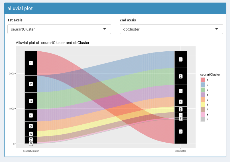
colData(scEx)$seurartCluster = as.factor(colData(scEx)$seurartCluster)comparing BiocSingular and Seurat PCA calculations:
-
Seurat
-
BiocSingular
pbm## An object of class Seurat
## 13713 features across 2638 samples within 1 assay
## Active assay: RNA (13713 features, 2000 variable features)
## 2 dimensional reductions calculated: pca, umap
# Assays(pbm)We have now created a SingleCellExperiment object with all information from Seurat. We will now try to recreate these results with SCHNAPPs:
We have to save the object in a file that can be opened with the “load” command.
To reproduce the results the following parameters have to be set in SCHNAPPs:
- Cell selection: ** Min # of UMIs = 1
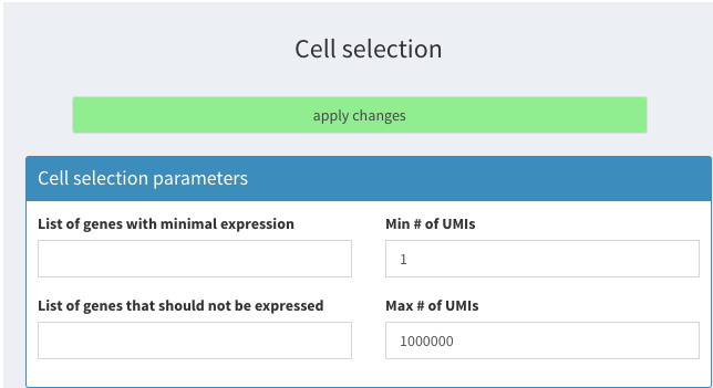
Cell selection parameters
Just to be complete (we will do this later) here is the list of cells that has to be removed:
AAAGATCTGGGCAA-1, AAAGCAGAAGCCAT-1, AACGCCCTGCTTAG-1, AAGGTCTGGTATGC-1, AATGTAACGTTTGG-1, AATTACGAGTAGCT-1, ACACAGACACCTGA-1, ACATGGTGCGTTGA-1, ACCTGGCTGTCTTT-1, ACTTAAGACCACAA-1, ACTTGTACCCGAAT-1, ACTTTGTGCGATAC-1, AGAGGTCTACAGCT-1, ATCACGGATTGCTT-1, ATTACCTGGGCATT-1, CACGCTACTTGACG-1, CAGTGTGAACACGT-1, CCAATGGAACAGCT-1, CCAGTCTGCGGAGA-1, CGACCTTGGCAAGG-1, CGAGCCGACGACAT-1, CGGAATTGCACTAG-1, CGTAACGAATCAGC-1, CGTACCACGCTACA-1, CGTACCTGGACGAG-1, CTAGTTTGAGTACC-1, CTCAGCTGTTTCTG-1, CTCATTGATTGCTT-1, CTGGCACTGGACAG-1, CTTAACACGAGCTT-1, CTTAAGCTTCCTCG-1, GAAAGATGTTTGCT-1, GAACGTTGACGGAG-1, GAATGGCTAAGATG-1, GACCATGACTCTCG-1, GACTGAACAACCGT-1, GCCACTACCTACTT-1, GCGAAGGAGAGCTT-1, GCTACAGATCTTAC-1, GGCACGTGTGAGAA-1, GTCAACGATCAGGT-1, GTGAACACAGATCC-1, GTGTCAGAATGCTG-1, GTTAAAACTTCGCC-1, TAAGATACCCACAA-1, TACGCAGACGTCTC-1, TACGCGCTCTTCTA-1, TACGGCCTGTCCTC-1, TATCACTGACTGTG-1, TCCCGATGCTGTGA-1, TCGCACACCATCAG-1, TCGTGAGAACTGTG-1, TGAAGCTGAGACTC-1, TGAGACACTGTGCA-1, TGAGCTGAGCGAGA-1, TGGAGACTGAAACA-1, TGGATGTGATGTCG-1, TGGCAATGGAGGGT-1, TGGTCAGACCGTTC-1, TGTTAAGATTGGCA-1, TTACTCGAACGTTG-1, TTCAAGCTTCCAAG-1
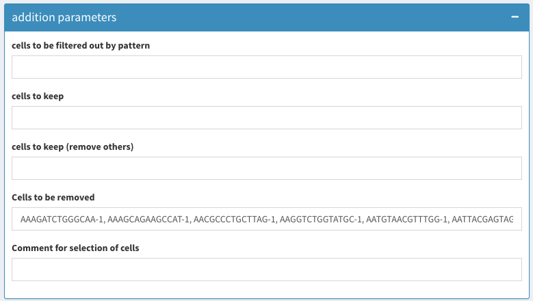
Cell selection additional parameters
- Gene selection ** remove regular expression ** set min expression to 1
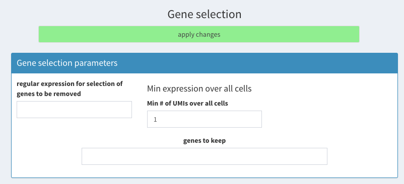
Gene selection parameters
- Parameters - Normalization
** Select SeuratLogNorm, the standard Normalization function in Seurat.
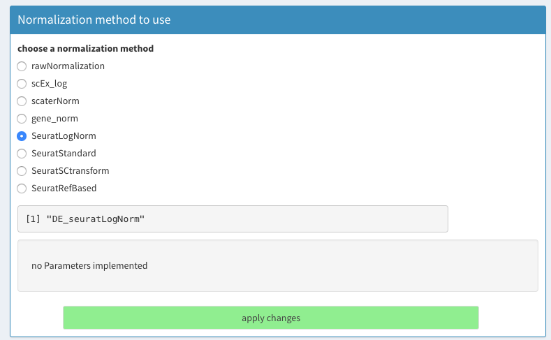
Select normalization method
Parameters - General Parameters
PCA parameters
** center = true ** scate = true ** use Seurat::RunPCA = ture ** Number of variable genes to be used = 2000 ** select highly expressed using “vst”
- Clustering parameters ** Seurat clustering tab. ** Dimensions from PCA to use: 10 ** k = 20
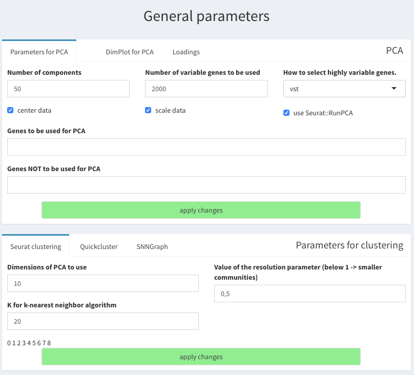
General parameters for PCA and clustering
- load input file
** unset sub sampling of data ** check “calculate normalization here”
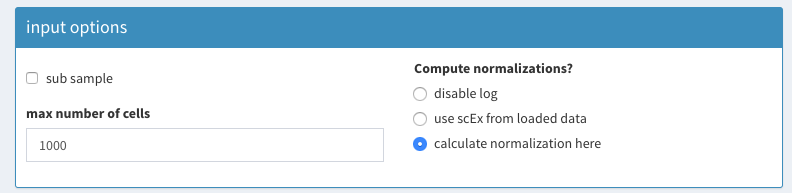
Load data - parameters
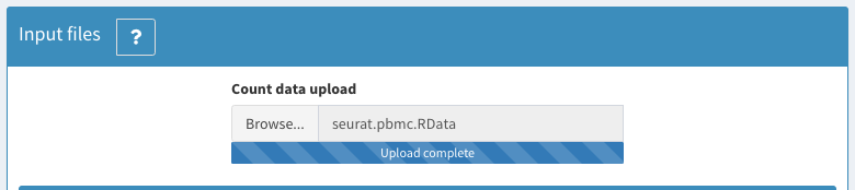
Load data select file
Set color for sample
Just for estetics:
Under Parameters - General Parameters set a nicer color for the samples other than black (which isn’t a color anyways.)
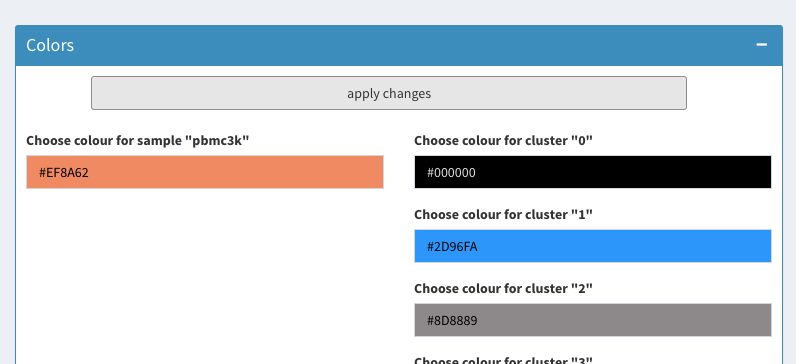
Set color for samples
select cells to be removed
Using the 2D plot the cells with more than 2500 nFeature_RNA and more than 5 percent.mt can be selected and removed from the data set:
We have to comply to three thresholds that are being used:
- nFeature_RNA > 200
- nFeature_RNA < 2500
- percent.mt < 5
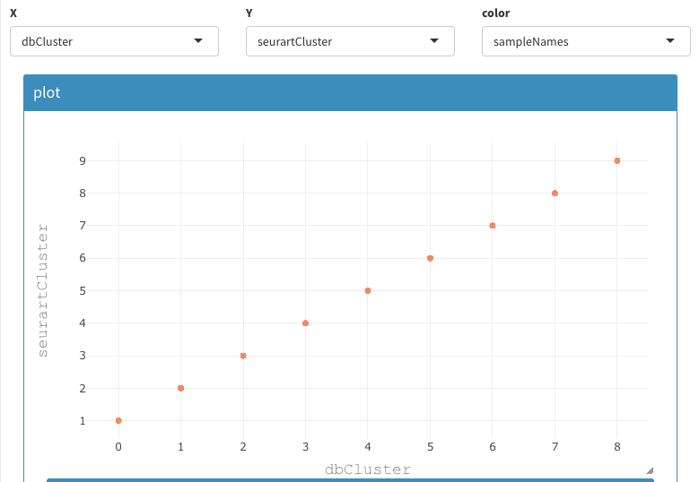
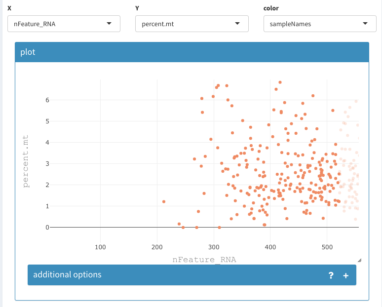
Go to Co-expression - selected:
set the following options:
- X : nFeature_RNA
- Y : percent.mt
- color: sampleNames
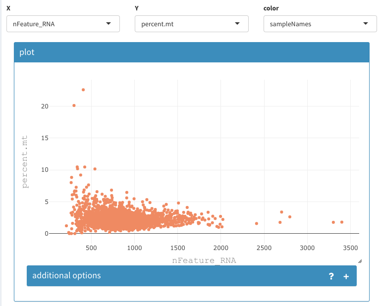
2D plot, select cells to be removed 1
select the zoom function in the plot:
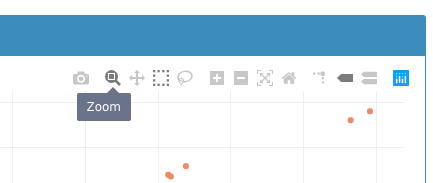
zooming selector
Zooming into the low nFeatureRNA region reveals that no cells will be removed using the 200 threshold.
Filter based on detected genes
choose box select:
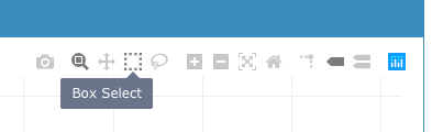
Selection tool (box)
- Select the cells that are higher than 5 (roughly) percent.mt
- set the name of the group to “rmCells”
- group names has to be plot
2D plot, select cells to be removed 2
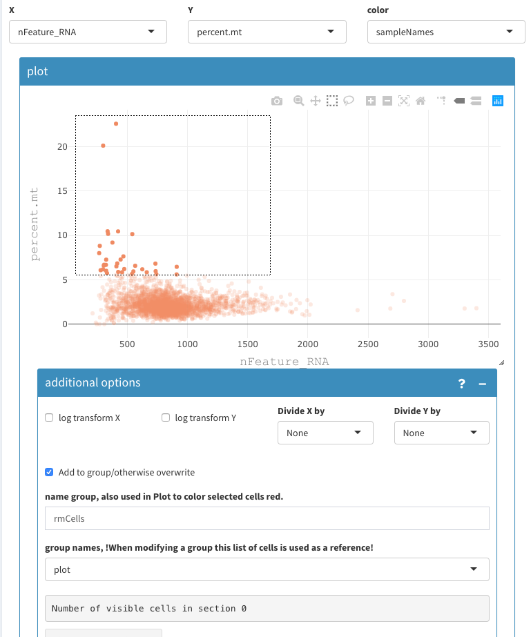
- click on current selection
=> the cells are now red
- set group names back to “plot”
change the zoom to be able to select anything around 5 percent.mt and show additional options:
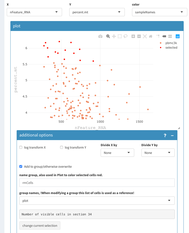
2D plot, select cells to be removed 3
- select the remaining cells and add them to “rmCells” list.
- if you are not sure about a cell the values can be shown hovering over the points
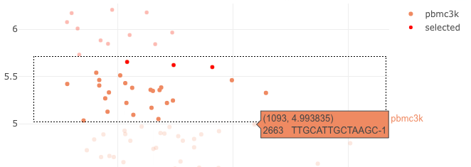
2D plot, select cells to be removed 4
- proceed similarly to select the cells that have more than 2500 nFeature_RNA.
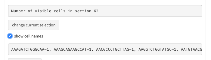
You should have 62 cells selected.
- check the “show cell names” check box.
- copy the cell names (tripple click on a cell name; Command-C)
- Paste the cell name under “Cells to be removed” (see above, cell selection)
- click “apply changes”
2D plot, select cells to be removed 4
- summary Stats:
That is how summary stats should look like:
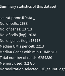
Summary statistics